In this post, I’m going to expand on the basics I laid out more informally here. I’m going to define some commonly used notation and key terms that I plan to use as other posts, so that this post can serve as a reference in the future. I may also add to it over time if I want to use more terms.
In general, we’ll be in settings where we observe \(n\) observational units. For each unit, indexed by \(i \in \{1, \ldots, n\}\), we’ll observe a vector of their covariates, \(\boldsymbol{X}_i\), and some response variable of interest, \(Y_i\). To give some examples:
- In measuring the lift of an ad campaign (or estimating the number of incremental conversions), the observational units could be individual people or households. The covariates \(\boldsymbol{X}_i\) could represent characteristics of the observational unit, like demographics and purchasing history. The response \(Y_i\) could represent how many purchases they made during an ad campaign, or their total spend.
- If a tech company wants to know whether the new version of their app increases engagement, the observational units would probably be individual users. The covariates could be user characteristics (like demographics and historic engagement) and the response could be some measure of engagement, like time spent in the app or number of likes/comments.
- If we’re trying to figure out the effect of a certain behavior on health, the observational units could be individual people. The covariates could represent demographics and medical history, and the response could be a health outcome like weight gain/loss or lifespan.
- When analyzing the impact of a law, the observational units could be individual states that each either pass a certain law or don’t. The covariates could be characteristics of the people in those states, like pre-study average income and crime rates. The response could be something that a law might plausibly effect, like post-study income or crime rates.
Most theoretical causal inference deals with a binary treatment—like receiving a medicine or a placebo, being reached by an ad campaign or not, whether or not a user downloaded the new version of the app, or whether or not the state passed a certain law. We’ll keep track of whether each observational unit was treated or not using the binary variable \(W_i\)—it will equal 1 for treated units and 0 for untreated units.
Potential Outcomes and Causal Estimands
In the Neyman–Rubin causal model, we assume that each observational unit has two potential outcomes—the outcome that would have occurred if their treatment was 0, \(Y_i(0)\), and the outcome that would have occurred if their treatment was 1, \(Y_i(1)\). So for every unit, we observe only the potential outcome corresponding to their actual treatment, \(Y_i(W_i)\). The other potential outcome, \(Y_i(1 – W_i)\), is unobserved.
An important thing to note here is that we’ll be thinking about our observed data as being a random sample from some kind of population. So \(\boldsymbol{X}_i, W_i\), \(Y_i(0)\), and \(Y_i(1)\) are all random variables. We’ll often want to do things like take their expected value (or average or mean), which I’ll denote by using the operator \(\mathbb{E}[ \cdot]\). Typically I’ll assume these units are independent and identically distributed (IID). (The combination of the IID assumption and the assumption that we observe \(Y_i(W_i)\) is sometimes called the stable unit treatment value assumption.)
The individual treatment effect for a single unit is most commonly defined as the difference between these two potential outcomes, \(Y_i(1) – Y_i(0)\). (Other definitions are possible; for example, maybe we’d care more about the ratio, \(Y_i(1)/ Y_i(0)\).) Notice that the individual treatment effect is also a random variable.
The basic reason why causal inference is hard is that no one has ever observed a treatment effect—we never get to see both the treated and untreated state for a single unit. This has, for good reason, been called the fundamental problem of causal inference. So it’s hard to validate whether our causal estimates are right or wrong. There are some ways to do it. But in general, since some of our assumptions are fundamentally untestable, making those assumptions as weak as possible is important in causal inference.
The individual treatment effect is the building block of most causal estimands. (An estimand is just a population characteristic we might want to estimate. Importantly, an estimand has to be a constant, not a random variable—at least in frequentist statistics.)
Maybe the most common causal estimand is the average treatment effect (ATE), \(\mathbb{E}[Y(1) – Y(0)]\). (The lack of subscript denotes that this is the expectation for a unit chosen at random from the population.) The ATE represents the expected individual treatment effect for a unit chosen at random from the population.
Another common estimand is the average treatment effect on the treated units (ATT), \(\mathbb{E}[Y(1) – Y(0) \mid W_i = 1]\). (Here the notation \(\mid W_i = 1\) denotes that this is a conditional expectation.) The ATT is the expected treatment effect among units that were treated.
If treatment was randomly assigned, the ATT is the same as the ATE. But if units have some say in whether or not they are treated, then the treated units might be systematically different than the untreated units, and could have a different treatment effect. More on that next.
Confounding
If treatment is randomly assigned (as in a randomized controlled trial or A/B test), estimating causal estimands is relatively easy. To estimate, say, the ATE, we can simply get the average outcome among treated and untreated units and take the difference of the averages.
If units have some say in whether or not they are treated, things become much trickier. Basically the issue is that there might be a systematic difference between units who are treated and units that aren’t. I referred to this as “selection bias” in my previous post, and you can read more about it there.
Here are some examples of when this happens.
- In an ad campaign, we might not randomly assign individuals or households to be reached. Or even if we do randomly assign units in some way, some units assigned to be reached might still not be reached—maybe they didn’t watch TV or open an app where they would have been reached.
- If a tech company wants to know the effect of downloading a new version of an app, they probably can’t make some people download the app or make others not download it. (Even if they have some ability to do this, they can’t control whether or not somebody opens the app at all during the study.)
- If we want to know the effect of a behavior like smoking on health, it might be unethical to assign some people to smoke.
- More generally, it might not be technically impossible to conduct a randomized controlled trial (RCT), but it might be prohibitively expensive or time-consuming. We might simply be unwilling to conduct an RCT, but nonetheless we’re still interested in the best estimate of a treatment effect that we can get without an RCT.
Mathematically, the problem with confounding is that the potential outcomes \(Y_i(0)\) and \(Y_i(1)\) are dependent on the treatment status \(W_i\). This is called confounding.
Unconfoundedness
A lot of causal inference has to do with figuring out ways to work around confounding. The most simple solution is pretty intuitive—figure out what all of the confounding variables are and control for them. This is much easier said than done, since we don’t always know what the confounding variables are, and we might not be able to observe all of them. But nonetheless it makes sense and is sometimes plausible.
We say that treatment assignment is unconfounded if the potential outcomes are conditionally independent of treatment status given the observed covariates. This assumption is also sometimes called strong ignorability or selection on observables.
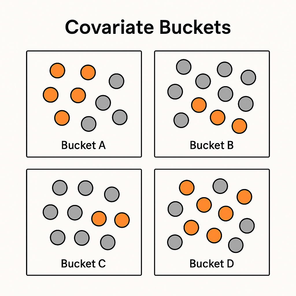
Here’s an intuitive explanation of what this means. Let’s say we’re trying to figure out the impact of an ad campaign on conversions. Let’s say the covariates we observe are all discrete, so we can divide all of our units into buckets, where in each bucket all of the units have all of the same covariates. Within each bucket, some of the units will be treated and some will not. If treatment assignment is unconfounded given our observed covariates, then which units in the bucket happened to be treated and which happened not to be treated is “as good as random.” There’s no systematic difference between treated and untreated units in the same bucket. In other words, within the bucket we’re safe to calculate the treatment effect for that bucket by taking the difference between the average outcome among treated units and the average outcome among untreated units.

One example of how this might fail would be if we didn’t control for income. All else equal, maybe people with higher incomes will have a higher likelihood of converting regardless of whether or not they’re reached. (In other words, the potential outcomes under being reached or unreached depend on income.) Maybe people with higher incomes are also less likely to be reached by an ad campaign—maybe people with higher incomes spend more hours of the day working and are exposed to fewer ads.
If so, then in our buckets that don’t control for income, there will be systematic differences on average between reached and unreached (treated and untreated) people. Higher income people will be under-represented among the reached units and over-represented among un-reached units. Since higher income people are also more likely to convert, it will look like the unreached units convert at higher rates than they really do, and we will underestimate the effect of the ad campaign on conversions.
Satisfying unconfoundedness can be really hard. And, it’s usually impossible to know for sure that you’ve achieved unconfoundedness because of the fundamental problem of causal inference. Doing your best to satisfy unconfoundedness is often more important than the particular estimator you choose that requires unconfoundedness.
Overlap
This brings up one more important assumption—overlap or positivity. This is the assumption that regardless of the value of the covariates, every unit has a positive probability of being treated or untreated. This assumption is important because in practice, we need to have at least one treated unit and untreated unit in every bucket, or else we can’t figure out the treatment effect within that bucket.