Estimating treatment effects with a linear model in a randomized experiment–insights from the Double/Debiased ML framework

When treatment assignment is randomized, one model that people often use for estimating treatment effects is \(y_i = \alpha + \boldsymbol{X}_i^\top \boldsymbol{\beta} + \tau W_i + \boldsymbol{\gamma}^\top W_i \cdot (\boldsymbol{X}_i – \boldsymbol{\overline{X}}) + \epsilon_i \) (sometimes called the ANCOVA II model), where \(W_i\) is the binary treatment indicator (1 if unit \(i\) is treated, 0 if not), \(\boldsymbol{X}_i\) is a vector of covariates for unit \(i\), and \(\boldsymbol{\overline{X}}\) is the sample mean of the covariates. Theorem 7.2 of Imbens and Rubin (2015) shows that if treatment is randomized (and basic regularity conditions are met) then the OLS estimator of \(\tau\) in this regression is a consistent and asymptotically normal estimator of the treatment effect.

Notably, this does not require the linear model in the covariates to be correct. This is perhaps a little mysterious. Normally in causal inference, we are very suspicious of assumptions unless they’re either mild regularity conditions or have an easy, plausible interpretation. That’s because unless we have randomized treatment assignment, we have to rely on fundamentally untestable assumptions to do causal inference. Worse, the consequences to our estimator of violating these assumptions is often unknowable–we’re writing a blank check. So, the general instinct is to keep these assumptions to an absolute minimum. Using a linear regression, which is almost certainly not the actual true model in most settings, goes against this instinct.

One hint of what’s going on is that the proof of Theorem 7.2 depends crucially on the assumption of randomized treatment assignment—unconfoundedness is not enough.¹

Recently I thought of another way to explore this concept of ANCOVA II’s robustness to misspecification. It has to do with augmented inverse propensity weighting, an estimator that also doesn’t require the outcome model to be correctly specified in order to get consistent and asymptotically normal estimation of the treatment effect.

A detour into AIPW/DML

The augmented inverse propensity weighting (AIPW) estimator for the average treatment effect is \(\hat\psi_{\text{AIPW}}
=\frac1n\sum_{i=1}^n\Bigl[
\hat m_{1}(\boldsymbol{X}_i)-\hat m_{0}(\boldsymbol{X}_i)\;
+\;
\frac{W_i\bigl(Y_i-\hat m_{1}(\boldsymbol{X}_i)\bigr)}{e(\boldsymbol{X}_i)}
-\frac{(1-W_i)\bigl(Y_i-\hat m_{0}(\boldsymbol{X}_i)\bigr)}{1-e(\boldsymbol{X}_i)}
\Bigr],\) where \(\hat m_{1}(\boldsymbol{X}_i)\) is a model for the treated potential outcome given covariates \(\boldsymbol{X}_i\), \(\hat m_{0}(\boldsymbol{X}_i)\) is the predicted untreated potential outcome, and \(e(\boldsymbol{X}_i) := \mathbb{P}(W_i = 1 \mid \boldsymbol{X}_i)\) is the propensity score.

Now in this setting, due to random assignment we know that \(e(\boldsymbol{X}_i) = 1/2\) for all \(i\) (or whatever the probability of treatment is, but let’s just go with \(1/2\) for simplicity).

Notice that if we use the ANCOVA II model, \(\hat m_{0}(\boldsymbol{X}_i) = \hat{\alpha} + \boldsymbol{X}_i^\top \boldsymbol{\hat{\beta}} \) and \(\hat m_{1}(\boldsymbol{X}_i) = \hat{\alpha} + \boldsymbol{X}_i^\top \boldsymbol{\hat{\beta}} + \hat{\tau} + \boldsymbol{\hat{\gamma}}^\top (\boldsymbol{X}_i – \boldsymbol{\overline{X}}) \).

In the spirit of double/debiased machine learning (DML), we can use a cross-fitting procedure to use the AIPW estimator with the ANCOVA II model. Here’s the connection that explains why I’m taking this detour: DML tells us that this cross-fit AIPW estimator \(\hat\psi_{\text{AIPW}}\) should also be consistent and asymptotically normal even if the linear model is misspecified (see why below).

Here’s the procedure:

1. Split the data into \(K \geq 2\) folds. (For simplicity, assume \(n/K\) is an integer, and every fold contains \(n/K\) observations.)
2. On fold \(k\), fit an ANCOVA II linear regression on all the data except for the observations in fold \(k\), yielding coefficients \((\hat{\alpha}^{(-k)}, \boldsymbol{\hat{\beta}}^{(-k)}, \hat{\tau}^{(-k)}, \boldsymbol{\hat{\gamma}}^{(-k)})\). Use it to model the response for the observations in fold \(k\).
3. Then construct the AIPW estimator from the results (simply plugging in the known \(e(\boldsymbol{X}_i) = 1/2\) for all the propensity scores): \(\hat\psi_{\text{AIPW}}
   =\frac1n\sum_{i=1}^n\Bigl[
   \hat m_{1}^{(-k(i))} (\boldsymbol{X}_i)-\hat m_{0}^{(-k(i))}(\boldsymbol{X}_i)\;
   +\;
   \frac{W_i\bigl(Y_i-\hat m_{1}^{(-k(i))}(\boldsymbol{X}_i)\bigr)}{1/2}
   -\frac{(1-W_i)\bigl(Y_i-\hat m_{0}^{(-k(i))}(\boldsymbol{X}_i)\bigr)}{1-1/2}
   \Bigr],\) where the notation \(m_{1}^{(-k(i))} (\boldsymbol{X}_i)\) denotes that for observation \(i\) we use the coefficients estimated without using the fold containing \(i\).

As I mentioned earlier, Theorem 7.2 told us that simply fitting the linear regression on the full data set would be enough for consistency and asymptotic normality of the OLS estimate \(\hat{\tau}\), even if the linear model isn’t correctly specified.

So then the question of this post is:

If we dig into it, can we see that this DML estimator \(\hat{\psi}_{\text{AIPW}}\) (derived from AIPW with the known treatment probabilities and the ANCOVA II outcome model) and vanilla ANCOVA II estimator \(\hat{\tau}\) are basically doing the same thing?

Since the propensity scores are a trivial constant, we might think that when we sort out the expression for \(\hat\psi_{\text{AIPW}}\) above, it might end up looking a lot like \(\hat{\tau}\). If this were true, since we already know that the cross-fit AIPW estimator is robust to misspecification of the ANCOVA II model, this would shed some light on why vanilla ANCOVA II is also robust to model misspecification.

By the way, why does the DML theory guarantee that this estimator is consistent for the treatment effect even under misspecification of the ANCOVA II outcome model?

Other than regularity conditions, the assumptions we need for this to work are:

1. Unconfoundedness (which we get automatically from random assignment)
2. Overlap (which we also have since the probability of treatment isn’t 0 or 1).

And the last thing we need to get consistency and asymptotic normality from Theorem 5.1 of Chernozhukov et al (2018) is for the product of the rates of convergence of the estimated propensity score and the estimated outcomes to be \(o(1/\sqrt{n})\). We have that, because the propensity scores are known, so they alone have expected errors that are \(o(1/\sqrt{n})\). So it doesn’t matter if the linear model is totally wrong—the errors on the outcome model could be \(O(1)\) and we’re still fine.

Now let’s sort out what that cross-fit AIPW estimator looks like.

Examining the cross‑fit AIPW estimator

Recall the generic AIPW score

\(\hat\psi_{\mathrm{AIPW}} =\frac1n\sum_{i=1}^{n} \Bigl[ \hat m_{1}^{(-k(i))}(\boldsymbol X_i)-\hat m_{0}^{(-k(i))}(\boldsymbol X_i) +\frac{W_i\bigl(Y_i-\hat m_{1}^{(-k(i))}(\boldsymbol X_i)\bigr)}{e(\boldsymbol X_i)} -\frac{(1-W_i)\bigl(Y_i-\hat m_{0}^{(-k(i))}(\boldsymbol X_i)\bigr)}{1-e(\boldsymbol X_i)} \Bigr].\)

Because treatment is assigned with probability ½,
\(e(\boldsymbol X_i)=\frac12\) for everyone, and

\(\frac{W_i}{e(\boldsymbol X_i)}-\frac{1-W_i}{1-e(\boldsymbol X_i)} = 2W_i – 2(1-W_i) = 2\bigl(2W_i-1\bigr).\)

On each fold we fit the centered ANCOVA‑II regression, so

\(\hat m_{0}^{(-k)}(\boldsymbol X_i)= \hat\alpha^{(-k)}+\boldsymbol X_i^\top\hat{\boldsymbol\beta}^{(-k)},\)
\(\hat m_{1}^{(-k)}(\boldsymbol X_i)= \hat\alpha^{(-k)}+\boldsymbol X_i^\top\hat{\boldsymbol\beta}^{(-k)} +\hat\tau^{(-k)}+\hat{\boldsymbol\gamma}^{(-k)\!\top}(\boldsymbol X_i-\boldsymbol{\overline X}^{(-k)}).\)

Substituting these into the score gives

\(\hat\psi_{\mathrm{AIPW}} =\frac1n\sum_{i=1}^{n} \Bigl[ \hat\tau^{(-k(i))} +\hat{\boldsymbol\gamma}^{(-k(i))\!\top}\bigl(\boldsymbol X_i-\boldsymbol{\overline X}^{(-k(i))}\bigr) +2\bigl(2W_i-1\bigr)\bigl(Y_i-\hat m_{W_i}^{(-k(i))}(\boldsymbol X_i)\bigr) \Bigr]\)

\(=\frac1K\sum_{k=1}^{K} \hat\tau^{(-k)} + \frac1n\sum_{i=1}^{n} \Bigl[ \hat{\boldsymbol\gamma}^{(-k(i))\!\top}\bigl(\boldsymbol X_i-\boldsymbol{\overline X}^{(-k(i))}\bigr) +2\bigl(2W_i-1\bigr)\bigl(Y_i-\hat m_{W_i}^{(-k(i))}(\boldsymbol X_i)\bigr) \Bigr],\)

the average of each of the \(K\) estimated \(\hat\tau^{(-k)}\) coefficients plus some other stuff.

Notice that the \(\hat{\boldsymbol\gamma}\)–term vanishes asymptotically: inside each split the covariates were centered, so \(\frac1n\sum_{i=1}^{n}\hat{\boldsymbol\gamma}^{(-k(i))\!\top}\bigl(\boldsymbol X_i-\boldsymbol{\overline X}^{(-k(i))}\bigr) \approx 0,\) and approaches 0 asymptotically. Hence this piece contributes nothing to \(\hat\psi_{\mathrm{AIPW}}\) as \(n\) gets large.

Last term

Now let’s look at the last term:

\(\frac1n\sum_{i=1}^{n} 2\bigl(2W_i- 1\bigr)\bigl(Y_i-\hat m_{W_i}^{(-k(i))}(\boldsymbol X_i)\bigr)\)

\(= \frac2n \bigl[ \sum_{\{i: W_i = 1\}} \bigl(Y_i-\hat m_{1}^{(-k(i))}(\boldsymbol X_i)\bigr) – \sum_{\{i: W_i = 0\}} \bigl(Y_i-\hat m_{0}^{(-k(i))}(\boldsymbol X_i)\bigr) \bigr]\)

If we were to fit ANCOVA-II on the full data set, the first-order conditions for OLS imply that \( \sum_{i=1}^n \bigl( y_i – \hat m_{W_i}(X_i) \bigr) = 0 \) and

\( \sum_{i=1}^n W_i \bigl( y_i – \hat m_{W_i}(X_i) \bigr) = 0 \)

\( \iff \qquad \sum_{\{i: W_i = 1\}} \bigl( y_i – \hat m_{1}(X_i) \bigr) = 0 ,\)

which combined with the above implies

\( \iff \qquad \sum_{\{i: W_i = 0\}} \bigl( y_i – \hat m_{0}(X_i) \bigr) = 0 .\)

So if you fit ANCOVA‑II on the whole data set, both of these last terms would have their difference equal to exactly zero. Asymptotically, with cross-fitting the same thing will happen–these terms are \(o_p(1/\sqrt{n})\).

Therefore, roughly speaking the AIPW estimator is simply

\(\hat\psi_{\mathrm{AIPW}}=\frac1K\sum_{k=1}^{K} \hat\tau^{(-k)} ,\)

the average of the \(K\) OLS-estimated coefficients for \(\hat{\tau}\). And in large samples, this will be roughly equivalent to estimating \(\hat{\tau}\) on the full data set.

I did some simulations that you can see below that illustrate that this works in practice. But first, let’s sum up what we’ve seen.

Takeaways

We have (informally) shown the asymptotic equivalence of the ANCOVA II estimator \(\hat{\tau}\) and the cross-fit AIPW estimator with ANCOVA II as the outcome model \(\hat\psi_{\mathrm{AIPW}}\) when treatment assignment is randomized.

This sheds light on the fact that ANCOVA II is consistent and asymptotically normal for the treatment effect even under model misspecification. Roughly speaking, the doubly‑robust structure needs either the propensity score or the outcome model to be correctly modeled. Here the propensity score is known, so any outcome regression—even a bad one—makes \(\hat\psi_{\mathrm{AIPW}}\) a consistent and asymptotically normal estimator.

As a result, in a randomized trial, cross-fit AIPW using ANCOVA‑II is doubly robust “for free’’: if the linear specification is right you get minimum variance; if it is wrong you still get consistency and asymptotic normality. And since it is asymptotically equivalent to vanilla ANCOVA II, it makes sense that ANCOVA II has the same asymptotic properties.

Simulation

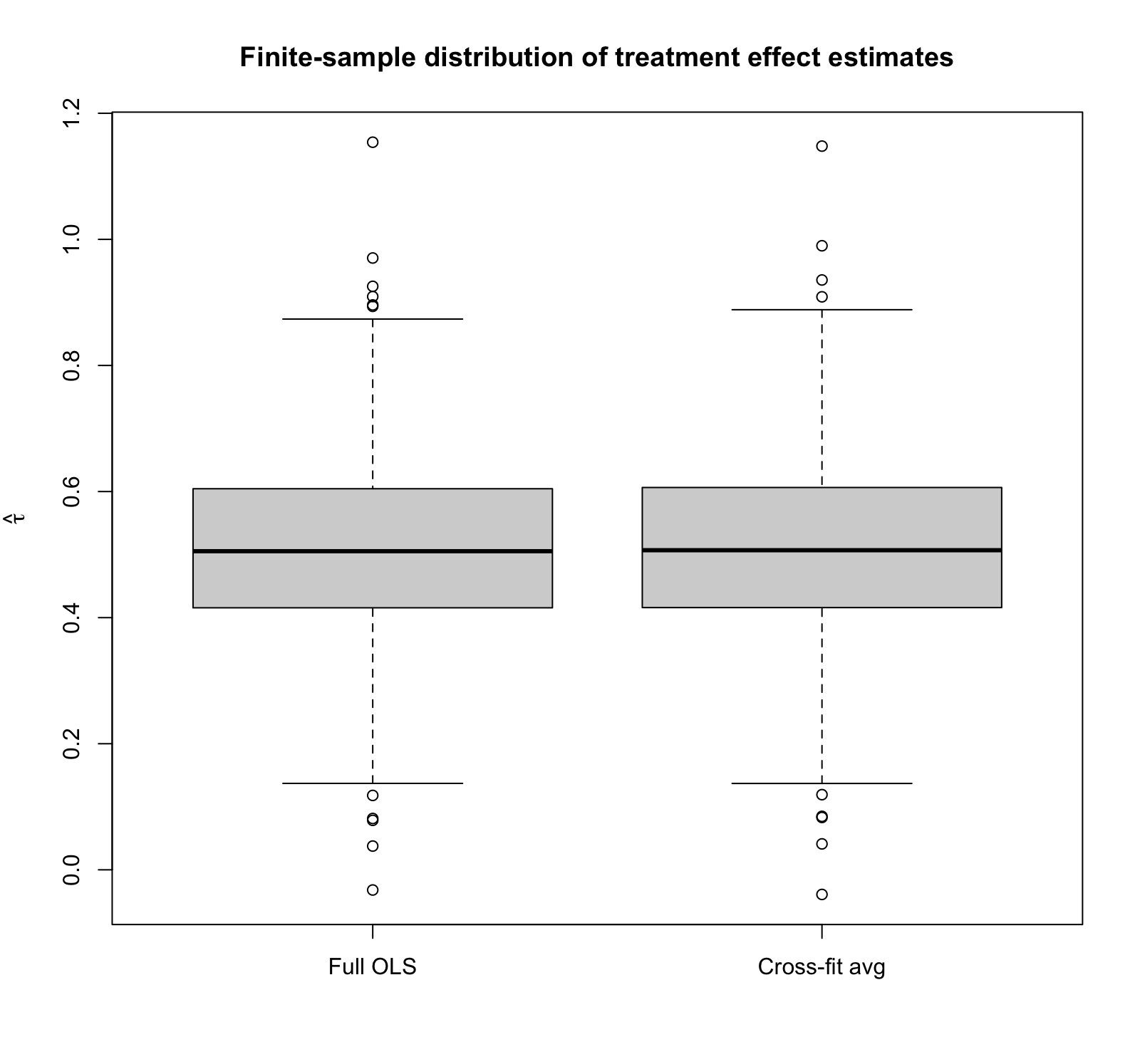
To illustrate the finite-sample results, I ran a 1000‑rep simulation study in which each replication generates \(n=400\) observations with five Gaussian covariates, assigns treatment by a fair coin, and produces outcomes from a deliberately non‑linear data‑generating process. For every replication I

1. Fit the centered ANCOVA‑II regression on the entire sample and record the OLS coefficient \(\hat\tau_{\text{full}}\)
2. Perform 5‑fold cross‑fitting, refitting the regression on the \(K‑1\) training folds each time, and
3. Compute the full cross-fit \(\hat\tau_{\text{cf}}\).

(See the complete code at the end of this post.) Note that the true treatment effect is 0.5. The box‑plot shows that the two sampling distributions are practically superimposed: both estimators are unbiased with means ≈ 0.50 and identical finite‑sample standard deviations (~0.148). In other words, even under blatant model misspecification, cross‑fitting buys you no accuracy and costs you no precision in a randomised trial, underscoring the asymptotic equivalence we just demonstrated analytically.

Notice also that we do seem to see outliers, suggesting that the finite-sample distribution of the estimator might not be Gaussian in this particular setting (so we haven’t fully hit the asymptotic regime), yet the two estimators still look nearly identical.

Estimator	Mean	SD
Full OLS	0.511	0.148
Cross-fit estimate	0.511	0.149

Bonus–what if we try a REALLY simple outcome model?

Since when we know the propensity score we don’t need the outcome model to be consistent—or even have decreasing errors—what if we just choose a fixed 0 for the outcome model? Will it still be consistent and asymptotically normal, like the theory says it should be?

In this case, the AIPW estimator becomes

\(\hat\psi_{\mathrm{AIPW}} =\frac1n\sum_{i=1}^{n} \Bigl[ 0 -0 +\frac{W_i\bigl(Y_i- 0 \bigr)}{e(\boldsymbol X_i)} -\frac{(1-W_i)\bigl(Y_i-0 \bigr)}{1-e(\boldsymbol X_i)} \Bigr]\)

\(\hat\psi_{\mathrm{AIPW}} =\frac1n\sum_{i=1}^{n} \Bigl[ \frac{W_i Y_i }{e(\boldsymbol X_i)} -\frac{(1-W_i) Y_i}{1-e(\boldsymbol X_i)} \Bigr],\)

which is the classical inverse propensity weighting estimator for the treatment effect. It’s consistent, and since we know the propensity scores, it’s simply

\(\hat\psi_{\mathrm{AIPW}} =\frac1n\sum_{i=1}^{n} \Bigl[ \frac{W_i Y_i }{1/2} -\frac{(1-W_i) Y_i }{1/2} \Bigr]\)

\( = \frac2n \bigl( \sum_{\{i: W_i = 1\}} Y_i – \sum_{\{i: W_i = 0\}} Y_i \bigr) ,\)

which is asymptotically normal, too. (Of course, we could get lower variance by at least attempting to model the outcomes, even if only with ANCOVA II.)

R Code

# --------------------------------------------------------
# Monte‑Carlo: full‑sample ANCOVA‑II vs. 5‑fold cross‑fit
# --------------------------------------------------------
rm(list=ls())
set.seed(42)        # reproducible randomness

R  <- 1000          # replications
n  <- 400           # sample size
p  <- 5             # number of covariates
K  <- 5             # folds for cross‑fitting

full_ols_tau <- numeric(R)   # store OLS τ̂
cfit_full_psi <- numeric(R)  # store cross‑fit τ̂

for (rep in seq_len(R)) {

  ## 1  generate data
  X <- matrix(rnorm(n * p), n, p)
  W <- rbinom(n, 1, 0.5)
  Y <- sin(X[, 1]) + X[, 2]^2 + 0.5 * W + 0.5 * rnorm(n)

  ## 2  ANCOVA‑II on the *full* sample
  Xc      <- sweep(X, 2, colMeans(X), "-")          # centre covariates
  design  <- cbind(1, X, W, W * Xc)                 # [1, X, W, W·Xc]
  coef_ls <- solve(t(design) %*% design,
                   t(design) %*% Y)                 # OLS via normal eq.
  tau_full <- coef_ls[1 + p + 1]                    # coefficient on W
  full_ols_tau[rep] <- tau_full

  ## 3  # K‑fold cross‑fit
  folds <- sample(rep(1:K, length.out = n))
  psi_hat   <- numeric(n)   # store per‑obs ψ̂

  for (k in 1:K) {
    idx_tr <- which(folds != k)
    idx_te <- which(folds == k)

    Xtr <- X[idx_tr, ]
    Wtr <- W[idx_tr]
    Ytr <- Y[idx_tr]

    # fit on training folds
    Xc_tr <- sweep(Xtr, 2, colMeans(Xtr), "-")
    Dtr   <- cbind(1, Xtr, Wtr, Wtr * Xc_tr)
    b     <- solve(t(Dtr) %*% Dtr, t(Dtr) %*% Ytr)

    # predictions for test fold
    Xte      <- X[idx_te, ]
    Wte      <- W[idx_te]
    Yte      <- Y[idx_te]
    Xc_te    <- sweep(Xte, 2, colMeans(Xtr), "-")   # center w.r.t training mean
    m0_hat   <- b[1] + Xte %*% b[2:(1 + p)]
    m1_hat   <- m0_hat + b[1 + p + 1] + Xc_te %*% b[(2 + p + 1):(2 + 2 * p)]

    psi_hat[idx_te] <- (m1_hat - m0_hat) +
      2 * (2 * Wte - 1) * (Yte - ifelse(Wte == 1, m1_hat, m0_hat))
  }

  cfit_full_psi[rep] <- mean(psi_hat)
}

## 4  summary table
summary_tbl <- data.frame(
  Estimator = c("Full OLS", "Cross-fit avg"),
  Mean      = c(mean(full_ols_tau), mean(cfit_full_psi)),
  SD        = c(sd(full_ols_tau),   sd(cfit_full_psi))
)
print(summary_tbl, digits = 3)

## 5  box‑plot
boxplot(list(`Full OLS` = full_ols_tau,
             `Cross-fit avg` = cfit_full_psi),
        ylab = expression(hat(tau)),
        main = "Finite-sample distribution of treatment effect estimates")

1. One way to explain this is that with pure observational data, the OLS residuals no longer have mean zero in treated/control groups. This causes ANCOVA II to lose robustness. ↩︎